In this example we want to analyze the reflective properties of a through silicon via (TSV) setup. This can be used in scatterometry tools as non-destructive measuring method to determine geometrical or material properties of the analyzed structure.
JCMsuite offers the possibility to efficiently compute shape and material derivatives of electromagnetic fields up to second order. Here, this feature is utilized to compute the dependence of the reflected Fourier coefficients on geometrical and material parameters of the structure. Since the derivatives are computed at little extra costs and are very accurate, their usage can greatly speed up assembling of libraries of scattering data or inverse data fitting procedures.
Shape derivatives
The layout of the TSV basically describes a periodic array of circular holes in a planar layer structure
In order to compute shape derivatives, the corresponding variable parameters have to be set in the layout file. Let us look at the relevant lines.
DerivativeParameter {
Name="Radius"
TreeEntry = "Layout3D/Extrusion/Objects/Circle/Radius"
}
DerivativeParameter {
Name="Height"
TreeEntry = "Layout3D/Extrusion/MultiLayer/Layer{2}/Thickness"
TreeEntry = "Layout3D/Extrusion/MultiLayer/Layer{3}/Thickness"
TreeEntry = "Layout3D/Extrusion/MultiLayer/Layer{4}/Thickness"
...
}
Layout3D {
Extrusion {
Objects {
...
Circle {
Radius = 70
DomainId = 2
GlobalPosition = [-200 -100]
RefineAll = 2
}
}
MultiLayer {
...
Layer {
Thickness = 40
DomainIdMapping = [1 4 2 4]
}
Layer {
Thickness = 70
DomainIdMapping = [1 2 2 1]
}
Layer {
Thickness = 50
DomainIdMapping = [1 3 2 1]
}
...
}
}
}
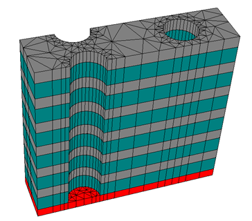
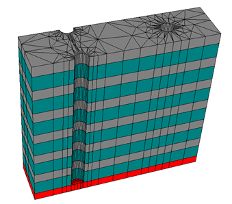
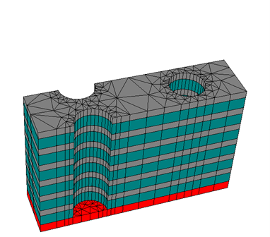
First two derivative parameters are defined in the DerivativeParameters section. The TreeEntry entries specify the geometrical quantities in the layout that should be effected by the parameter. The following figure shows the geometry when the “Radius” and“Height” parameters are changed:
Material derivatives
Definition of variable materials is done in the materials file. The syntax is similar to shape parameters:
DerivativeParameter {
Name = "NLayer"
TreeEntry = "Material{2}/RelPermittivity/RefractiveIndex/N"
}
DerivativeParameter {
Name = "KLayer"
TreeEntry = "Material{2}/RelPermittivity/RefractiveIndex/K"
}
...
Material {
DomainId = 2
RelPermittivity {
RefractiveIndex {
N = 1.31
K = 0.0
}
}
RelPermeability = 1.0
}
We defined the permittivity by specifying real and imaginary part of the refractive index. The Derivative Parameters effect those values. I.e. the parameter “NLayer” changes the real part of the refractive index of Material 2, and “KLayer” the imaginary part.
Scattering project with derivatives
After definition of the derivative parameters, we activate their computation in the project file:
Project {
InfoLevel = 3
Derivatives {
Order = 1
}
Electromagnetics {
TimeHarmonic {
Scattering {
Accuracy {
Precision = 0.02
}
}
}
}
}
by simply specifying the derivative Order in the Derivatives section. The order can be increased to 2, which allows for second-order partial derivative computation. Or it can be set to 0, which disables derivative computation. Looking at the solver output, we can check the reported computation of derivatives
updating inner nodes and computing first derivatives (4 parameters) ...
The incoming field are plane waves with 10deg oblique incident angle and 500nm wavelength for two orthogonal polarizations:
SourceBag {
Source {
ElectricFieldStrength {
PlaneWave {
K = [0.0, 2182127.35707073, -12375459.2082457]
Amplitude = [1.0, 0.0, 0.0]
}
}
}
}
SourceBag {
Source {
ElectricFieldStrength {
PlaneWave {
K = [0.0, 2182127.35707073, -12375459.2082457]
Amplitude = [0.0, 0.984807753012208, 0.173648177666930]
}
}
}
}
In a post process we compute the Fourier coefficients in upper direction, i.e. NormalDirection = Z:
PostProcess {
FourierTransform {
FieldBagPath = "project_results/fieldbag.jcm"
OutputFileName = "project_results/fc.jcm"
NormalDirection = Z
Format = JCM-ASCII
}
}
When derivatives are computed in the scattering project, all post processes automatically handle these derivative fields, e.g. computing the derivatives of Fourier coefficients with respect to the 2 geometrical and 2 material parameters in this example.
The Fourier coefficients result file has additional columns for each parameter derivative with the corresponding derived quantities, e.g. d(Electric FieldStrength X_1)_Radius f or the derivative of the x-component of the Fourier mode with respect to parameter “Radius”.
|
